Trajectory IK in Newton
newton.ik.IKSolverTrajectory solves every frame of a joint trajectory jointly — one nonlinear least-squares problem over all frames — instead of frame by frame. Existing per-frame objectives work unchanged; new temporal objectives couple consecutive frames and make the system block-banded, which is what the GPU solve exploits.
What was added
IKSolverTrajectory— Levenberg–Marquardt over all frames of one or more trajectories; rows are (trajectory, frame); damping and accept/reject are per-trajectory; the wholestep()is CUDA-graph capturable.- Temporal objectives —
IKObjectiveSmoothness(velocity / acceleration / jerk in tangent space),IKObjectiveVelocityLimit,IKObjectiveJointReference. They report bounded per-frame-offset Jacobian blocks; no global Jacobian is ever materialized. - Per-frame objectives reused unchanged — position / rotation / joint-limit
objectives (and all three Jacobian modes) just get one target per frame. Frames can be pinned
exactly via
fixed_frames. - Free-joint correctness — floating-base linear rows carry the exact [p]× lever-arm coupling of Newton's world-frame tangent convention (finite-difference-verified far from the origin).
- Dynamics-aware objectives —
IKObjectiveGravityTorque(minimize the static holding torque; dense analytic gravity-Hessian blocks) andIKObjectiveApparentGravity(the "waiter" objective: keep apparent gravity aligned with a carried surface's normal; task-space stencil-2 blocks). Both validated againsteval_inverse_dynamics/ finite differences and, for the waiter, a MuJoCo forward simulation. See the two sections below, andpython -m newton.examples ik_waiterfor the interactive ball-on-plate demo.
Why it's fast: the problem is block-banded
Per-frame costs touch one frame; smoothness costs touch k+1 consecutive frames. So the Gauss–Newton Hessian is block-banded — tridiagonal for velocity costs, wider for acceleration/jerk — and the Newton step costs O(T), not O(T³).
Batched block-tridiagonal Cholesky
- Block Thomas: one CUDA block per trajectory, sequential over frames inside a single
wp.tile_choleskykernel — exact solve. - Higher-order stencils reblocked into k·n superblocks, so accel/jerk costs reuse the same tridiagonal kernel.
- Sequential-in-T cost hidden by batch parallelism: 64 trajectories cost about the same as one.
Block-Jacobi preconditioned CG
- Block-banded Hessian in BSR form (
warp.sparse, fixed topology, values rewritten in place) + batchedwarp.optim.linear.cg. - Hand-rolled block-Jacobi preconditioner (per-frame n×n blocks inverted with
tile_cholesky_solve), warm-started across LM iterations. - Parallel over frames — wins for long horizons; inexact but agrees with direct to ~1e-6.
SPIKE: parallel-in-time direct
- Partitions the horizon; interiors factorize in parallel (one CUDA block per partition per trajectory) with the spike columns as extra right-hand sides.
- Symmetric Schur complement on the interface blocks — stays SPD, so the reduced system reuses the same Cholesky kernel. Exact: digit-identical LM traces to direct.
- Sequential depth O(T/P) instead of O(T): 5.8× faster than direct at T=960, 12.6× at T=3840.
ICRA-style writeup
- Full paper draft (PDF) — formulation, the three backends, cross-library benchmarks with an explicit timing taxonomy, and the G1 retargeting case study.
Results — trajectory solve
Shared task: Franka FR3, T=120 frames @ 30 fps, 4 trajectories, end-effector path through
pick-and-place waypoints, 16 LM iterations, analytic Jacobians. The frame-by-frame baseline is the
per-frame IKSolver, warm-started and batched across the 4 trajectories.
The full timing grid: batch × horizon, both robots
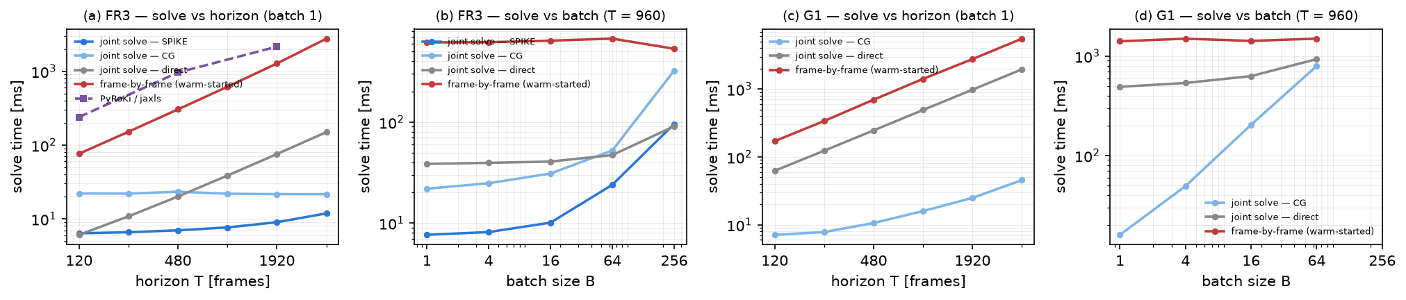
Filling in the coverage between the spot benchmarks above: steady-state whole-trajectory solve time over T ∈ {120…3840} × B ∈ {1…256} for every applicable backend, at equal 16-iteration budgets on identical FK-feasible targets. On the arm, SPIKE is the fastest backend everywhere beyond the smallest problems (direct edges it by <10% at T=120 and at B=256 for T≤960, where batching already saturates the GPU) — 12.6× over the sequential direct sweep and 233× over the warm-started per-frame loop at (T=3840, B=1); an equal-iteration PyRoKi/jaxls run of the identical problem trails even the per-frame loop (239× vs SPIKE at T=1920; the 12× headline elsewhere on this page is the equal-quality protocol, which lets jaxls terminate early). On the humanoid, CG leads at small batches (88× over per-frame at T=960 B=1, 43× over direct at T=3840) while direct becomes competitive at large batches (1.2× faster than CG at T=240, B=256) once batch parallelism hides its serial depth. The per-frame loop is flat in B — batching rescues most of its throughput gap (to within 1.9× of CG at B=64) but not its greedy quality. SPIKE sits out the G1 rows (the m=35 shared-memory cap); PyRoKi sits out G1 (no off-the-shelf floating-base variable in jaxls, same reason the single-frame comparisons used fixed-base H1).
Humanoid retargeting (G1, soma-retargeter data)
soma-retargeter today drives newton.ik frame by frame to retarget human motion
(it produced the G1 motions in BONES-SEED). Same front end here — SOMA BVH clips scaled to 14
world-frame effector targets — but the whole clip is solved jointly on a floating-base
29-DoF G1 (free joint, so the lever-arm coupling matters).
Torque-aware IK: minimize the gravity load, not just the path
Kinematic smoothness says nothing about effort. Two additions couple the trajectory
solve to the robot's dynamics. The first, IKObjectiveGravityTorque, penalizes the
static holding torque g(q) = ∂U/∂q at every frame — a stencil-0 temporal
objective whose dense coefficient block is the analytic gravity Hessian, assembled from subtree
mass aggregates and the batched world motion subspace (unactuated floating-base DoFs contribute
zero rows). On a Franka carrying 3 kg along a fixed end-effector path, it visibly
re-postures the arm and takes the binding shoulder joint from 83% to 61% of its torque limit
for a ~25 mm tracking concession; post-hoc torques are verified with Newton's
eval_inverse_dynamics (M, Coriolis and gravity terms, central-difference q̇, q̈).
Honest caveat: manipulator torque limits are generous (a stock FR3 does this task at 83% of its shoulder limit with smoothing alone), so "avoid the limit" only bites with heavy payloads or de-rated drives. The better framing is effort/heat: mean |τ| drops 5–19% here (mechanical energy stays roughly flat — the payload's potential-energy profile is fixed by the path), and the objective composes with everything else in the solve.
Balance-aware IK: the waiter problem, validated in simulation
The second addition, IKObjectiveApparentGravity, is a task-space temporal
objective (stencil 2): it penalizes the tangential components of the apparent specific force
f = aee − g felt by a surface carried on a link, with
aee the second difference of the carried point and the tangent axes evaluated
mid-stencil. Its Jacobian combines the acceleration stencil projected on the plate tangents
with a plate-tilt term — so the solver both smooths the carried point's acceleration and
banks the plate into the motion, like a waiter with a loaded tray. The banded assembly
already supports the dense task-space blocks; the objective just pads its two residual rows to
the temporal block size.
Validation runs the loop the objective only approximates: the IK output drives a PD-controlled Franka in a MuJoCo forward simulation carrying a plate with a free ball on it (elliptic friction cone, no cheats). With a level-plate orientation objective the dash flings the ball off; with the apparent-gravity objective the plate banks and the ball stays.
The batch-one extreme: million-frame toolpaths with SPIKE
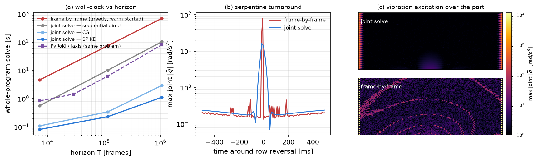
Corpus retargeting saturates the GPU with batch parallelism, so the horizon-parallel SPIKE backend adds nothing there. Its home turf is the opposite regime: one very long trajectory, fully known before execution — prescribed manufacturing paths. Laser marking and texturing, robotic additive manufacturing, spray coating, and ultrasonic scan coverage all fit: the whole program exists in advance, horizons reach millions of frames, and the arm is low-DoF, which keeps SPIKE's superblocks inside the tile shared-memory budget (the same cap that rules it out on the 35-DoF G1).
The demo engraves a raster image onto a domed panel with an FR3: every pixel sample is one
frame of a serpentine toolpath, and the tool is axisymmetric, so a new
IKObjectiveAxisAlignment objective points the flange axis along the surface normal
while leaving the spin free as redundancy. A 1152×912 raster is a
T = 1,050,624-frame trajectory — 2.4 hours of execution at
120 Hz — solved as one nonlinear problem (32 LM iterations, ~9 GiB):
| solver | whole-program solve | mean tracking | mean jerk |
|---|---|---|---|
| joint solve — SPIKE (P=1094) | 1.1 s | 0.01 mm | 1 |
| joint solve — CG | 2.9 s | 0.01 mm | 2 |
| PyRoKi / jaxls, same formulation & budget | 81.3 s (+ 91 s XLA compile) | 0.01 mm | 1 |
| joint solve — sequential direct | 103.7 s | 0.01 mm | 1 |
| frame-by-frame (16 iters/frame, warm-started, graph-captured) | 701 s | 0.00 mm | 5 |
Everyone tracks at hundredths of a millimeter — the differences are dynamics and latency. A jaxls/PyRoKi formulation of the identical problem (custom axis cost, same weights and iteration budget) lands at 73× the SPIKE time — and to its credit, it does complete the million-frame solve. The greedy per-frame loop carries a 5× acceleration spike into every serpentine reversal, and more damagingly it converts the image content itself into joint-jerk ripple: the engraved figure is literally visible in its vibration-excitation map, exactly where marking quality matters. The joint solve pre-shapes the reversals and confines excitation to the off-image turnaround margins. And the whole-program latency is the workflow win — re-pose the workpiece, re-solve the entire 2.4-hour program in about a second, and check reachability and clearances interactively instead of as a batch job.
Scaling up: all of BONES-SEED on one GPU
The BONES-SEED dataset — 288 hours of motion, 142,220 clips at 120 fps, with G1 retargets produced by soma-retargeter's production per-frame loop — is the corpus-scale stress test. The whole dataset streams from its tarball (never extracted) through a vectorized BVH front end (exact-parity rewrite of soma's loader, ~10× faster) into length-bucketed batched trajectory solves of 64 clips at a time. End to end: ~3.0 hours on this box's single GPU — preprocessing all 124.5M frames takes 21 minutes with zero errors, the joint solve of all 142,220 clips the remaining 160 — versus ~15 hours projected for the production-style batched per-frame loop at its measured rate on the same GPU. (The corpus tail is brutal: the longest 8% of clips hold 25% of the frames, and earlier runs silently lost them to a solver-rebuild OOM that the final pipeline fixes.)
Where the speedup numbers come from
Different comparisons at different scales measure different things — this table is the reconciliation. The hundred-fold numbers compare our frame-parallel solve against the production pattern at its worst utilization: one clip, sequential over frames, no batching (the honest latency story — one clip in flight is exactly the interactive case, where frame-by-frame has no batching available). Batching 100 clips rescues frame-by-frame's GPU utilization; what it cannot rescue is the serial chain over frames. Batched-vs-batched, the joint solve is 10× on solve throughput and 5.5× end-to-end — and 5.5× is conservative twice over: the projection charges the per-frame loop for pure solve only (no disk IO, no readback, no writes) while our 160 min includes everything, and the joint solve now also carries the full contact/guard objective set that the production loop doesn't have. Notably the joint solve does more arithmetic per frame (40 LM iterations touching every frame + 16 CG iterations, vs 24 per-frame iterations): the win is utilization and launch amortization — one captured mega-graph over 57k frames versus ~105 sequential small launches with host round-trips.
| comparison | joint solve | frame-by-frame | ratio | what each side is |
|---|---|---|---|---|
| FR3, 120 frames × 4 trajs | 2.7 ms replay / 17.9 ms cold | 715 ms | 265× / 40× | both batched across the 4 trajs, 16 iters both sides |
| G1 dance, 690 frames | 206 ms | 29.5 s | 143× | FBF one-clip sequential, 24 iters/frame, warm-started |
| G1 walk, 1088 frames | 213 ms | 46.3 s | 217× | same; targets exceed leg reach (workspace-boundary chatter) |
| corpus solve rate | 24,336 f/s | 2,378 f/s | 10.2× | both batched (B=64×896 frames vs B=100), graph-captured vs per-frame stepped |
| corpus wall-clock | 160 min measured | 873 min projected | 5.5× | ours end-to-end incl. all IO and the full objective set (v6); theirs pure-rate extrapolation |
Quality is a genuinely two-sided story, so it gets the full protocol treatment (foot
sliding/floating during source-labeled contact, ground penetration, smoothness, joint limits,
keypoint faithfulness — conventions from ReActor/OmniRetarget/PHC/GMR). A qualitative audit of
the comparison viewer caught real problems in earlier configs — an over-smoothed baseline with
locked elbows, shoulder/elbow branch flips, and an LM stall on clips far from the world origin
— root-caused to a free-joint tangent-convention mismatch whose Jacobian error grows with
distance from the origin, and fixed upstream in the solver with body-centered base tangents
(the pipeline keeps xy-centering and a symmetry-breaking seed as defense in depth; the
flagged retry tail shrank from 111 clips to 21 across the whole corpus). The
current numbers — the full 142,220-clip corpus solve (v6, quality-identical to v5 after
the solver speedups), evaluated on the standard
14,222-clip subset: the plain retuned joint solve tracks to 10.7 mm at 5.7× lower
peak acceleration than production. Adding the ported objectives — world-plane penalties on
foot points plus a whole-body capsule-surface guard
(IKObjectiveWorldPlaneCapsule, radii fitted to the G1 collision meshes),
contact-gated stance pins (IKObjectiveFootContact +
IKObjectiveFootSkate), and a rest-pose anchor
(IKObjectiveJointReference, the branch-flip fix) — brings key-effector error to
1.9 mm (production: 1.4) with foot slide at 2.3 cm/s (production:
2.2), foot penetration below production's own rate (1.3% vs 3.7% of frames),
and a 2–3× smoothness advantage. Body-surface contact is no longer a blind spot:
penetration is now also measured over a per-link capsule set fitted to the G1 collision
meshes, and there too the joint solve comes in below the production data (3.9% vs 5.2% of
frames, at less than half the mean depth). The remaining body contact is concentrated in
floor work (kneeling, crawling, sitting), where the scaled human pelvis target sits lower
than the robot's own thigh radius allows — tracking and the surface guard trade off, and the
viewer shows the equilibrium faithfully.
→ Open the side-by-side comparison viewer — the SOMA human source next to the shipped production retarget, our plain joint solve, and the joint solve with ported objectives, animating in sync on 13 curated clips. Watch the crawling and kneeling clips: production (which has no contact handling) digs into the floor; the plane objective holds ours out. Built on the Apache-2.0 seed-viewer's model assets.
Walking the accuracy–smoothness frontier
Is the quality table above one fixed tradeoff, or a knob? A knob: scaling the smoothness weights by λ while holding the contact/plane objectives fixed traces a frontier of tracking error against acceleration/jerk, re-solved on the 14,222-clip evaluation subset (~25–35 minutes per point on one GPU). Frame-by-frame solving has no such knob — its temporal regularity is whatever warm-starting leaves behind, and its acceleration spikes are noise, not a chosen tradeoff: points below this frontier.
Cross-library check: single-frame IK still holds up
Re-run of the earlier single-frame comparison (Newton IK paper protocol: random reachable targets from FK of uniform-random configurations; success = position < 5 mm and orientation < 0.05 rad). Original numbers were measured on an RTX 4090; these are on this box's RTX PRO 6000, so compare ratios, not absolutes.
Appendix
Design space: who solves the banded system how
Everyone in trajectory optimization sits at one of four points on how they solve the block-banded Gauss–Newton system (bandwidth 2(k+1)n−1 for k-order costs; the banded Newton step is O(T·k²n³) — linear in T, same structure as Riccati/DDP and factor-graph message passing):
| Approach | Who | Linear algebra | Parallel over T? | Batch? |
|---|---|---|---|---|
| Direct banded / Riccati | KOMO, GPMP2, Crocoddyl/Aligator, OCS2 | banded/block-tridiag Cholesky, exact | no (sequential sweep) | rare (CPU) |
| Iterative CG on normal eqs | pyroki/jaxls, MPCGPU | matrix-free or BSR SpMV | yes | yes |
| Quasi-Newton, no linear solve | cuRobo (L-BFGS on B-spline knots) | two-loop recursion only | yes | excellent |
| Sampling | STOMP, MPPI, MJPC | none | rollouts parallel | excellent |
Newton's prototype ships the first two as selectable backends (direct is new territory for GPU-batch; jaxls has no banded direct solver — its only sparse direct option is CHOLMOD via a CPU host-callback). cuRobo never forms a Jacobian: temporal structure lives in its B-spline knots (16 knots × 7 DoF = 112 variables, small enough that sparsity stops mattering), with linear-ish convergence and ~100 fixed iterations in exchange. Parallel-in-time direct methods (associative-scan LQR, cyclic reduction) exist but only pay off for single very long trajectories; batch parallelism is the cheaper GPU win.
Warp assessment: what worked, gaps, proposed extensions
Worked out of the box (pinned 1.15.0.dev)
tile_cholesky/tile_lower_solve/tile_matmulcompose into a batched banded factorization inside one kernel with a runtime-length sequential loop — including CUDA graph capture (~0.9 ms for 256 T=240 n=8 tridiagonal solves).- BSR construction + in-place value rewrites (
bsr_from_triplets,bsr_block_index), batched CG (batch_offsets), capturablecheck_every=0loop. No warp fork needed.
Gaps & bugs hit
preconditioner(A, "diag")is point-Jacobi even for block BSR — block-Jacobi was hand-rolled (~60 lines).- Bug (pinned version; fixed on warp main): iterative solvers' internal reductions don't pass
device=— CPU solves return NaNs when the default device is CUDA. Worked around withwp.ScopedDevice. - No direct sparse factorization of any kind in warp — the tile API is the only route (fine for banded, rules out general sparsity).
- Tile shapes are compile-time: one specialization per (DoFs, residuals, bandwidth); first-use JIT is 30–60 s per combination.
- Shared memory bounds the superblock (k·n ≲ 64–96 fp32) — jerk-order smoothing on high-DoF humanoids needs the non-reblocked banded variant or the CG path.
Small warp extensions worth proposing
preconditioner(A, "block_diag")for BSR.block_tridiag_cholesky(D, L, b, x)on (B,T,n,n) arrays — the canonical trajopt/Kalman/spline kernel this branch effectively contains.bsr_diag_add(A, λ)for LM damping; deterministic transpose SpMV; per-batch early exit in batched iterative solvers.
Benchmark protocol & caveats
- Hardware: all new numbers from this page: RTX PRO 6000 Blackwell (sm_120), driver 595.84. The reference single-frame numbers (shown hollow) are from the Newton IK paper on an RTX 4090 — absolute times are not comparable across the two GPUs; the cross-solver ratios are the signal.
- Single-frame: Newton = 64 Roberts seeds, 16 LM iterations, analytic
Jacobians, CUDA graph (asv protocol). cuRobo = v0.7.8 source build, its own published
benchmark config (
franka.yml, 16 seeds, CUDA graphs, collision checking off). PyRoKi = current pyroki/jaxls, same URDFs as Newton (FR3; plain 19-DoF H1 with 4 EE targets: both elbows + both ankles). Median of 10 runs after warmup; JIT/compile excluded. - Robot models differ slightly across libraries (cuRobo uses its packaged Panda; Newton/PyRoKi use FR3) — inherited from each library's standard config, same as the original comparison.
- Trajectory task is identical for Newton and PyRoKi (same URDF, targets, weights, T=120@30fps, frame 0 pinned; Newton 16 LM iterations, jaxls run to its own convergence). cuRobo's trajectory optimizer solves start→goal motion generation on B-spline knots — not full-path tracking — so it is reported as context, not a head-to-head.
- Trajectory tracking error: the joint solve trades tracking against smoothness by design (weights: pos 1.0, rot 0.5, limits 10, vel 0.01, accel 5e-4, rest-pose 1e-3). The frame-by-frame baseline tracks near-exactly but with ~3× the peak acceleration and jerk. Longer horizons traverse the same path more slowly, so both error and smoothness improve with T.
- G1 retargeting: soma-retargeter front end (SOMA BVH → scaled 14-effector targets, its production ik_map weights), 30 fps downsample, floating base. Frame-by-frame baseline = 24 warm-started iterations per frame (soma production setting); trajectory = 16 LM iterations, velocity+acceleration smoothness replacing the per-frame smoothing filter, without soma's foot-contact post-processing on either side.
Pointers
- Branch:
dylanturpin/newton-collab @ dylanturpin/trajectory-ik - Demo:
python -m newton.examples ik_trajectory - Design notes:
TRAJECTORY_IK_NOTES.md(design space, warp assessment, next steps) - Solver:
newton/_src/sim/ik/ik_trajectory_solver.py· objectives:ik_trajectory_objectives.py· tests:test_ik_trajectory.py - Benchmarks & this page:
traj_ik_report/on the same branch (git-excluded)